Understanding Computational Complexity

A Comprehensive Guide to Algorithm Performance Analysis

CS 101 - Spring 2026

On For Today

Let’s explore algorithm complexity!

Topics covered in today’s discussion:

⚡ O(1) - Constant Time — Lightning-fast operations that never slow down
🔍 O(log n) - Logarithmic Time — Divide and conquer excellence
🏥 Heap-Based Structures — Smart priority management
💥 O(2^n) - Exponential Time — The recursive explosion
🗺️ Travelling Salesman Problem — Real-world optimization challenges
📊 Performance Comparison — Understanding when to use each approach

Why Algorithm Complexity Matters

Important

Real-World Impact

Understanding algorithm complexity helps you:

⚡ Build Faster Software — Choose the right algorithm for the job
💰 Save Money — Efficient code means lower server costs
🌍 Scale Applications — Handle millions of users smoothly
🔋 Reduce Energy Usage — Green computing through efficiency
🎯 Make Smart Trade-offs — Balance speed, memory, and complexity

Note

The Big Idea: Small algorithmic choices can mean the difference between a program that runs in seconds versus one that takes years. Let’s explore how different complexity classes affect real-world performance!

Part 1: O(1) - Constant Time

The Speed Champion ⚡

O(1) means the algorithm takes the same amount of time regardless of input size!

Key Insight: Think of O(1) operations like light switches 💡. Whether you have 1 light or 1000 lights in your house, each switch always takes the same time to flip!

What is O(1) - Constant Time?

The Superpower of Algorithms ⚡

O(1) means the algorithm takes the same amount of time no matter how much data you give it!

Real-World Analogy: * Like a valet parking service - you hand over your ticket and get your car back instantly * Whether there are 10 cars or 10,000 cars in the lot, it takes the same time! * The valet has a direct system to find your exact car

Performance Guarantee 📊

10 items → 1 step
100 items → 1 step
1,000,000 items → 1 step
Same speed forever!

Key Insight 🔑

The algorithm has a “shortcut” that goes directly to the answer without checking other data!

Magic Question:

“Can I get the answer without looking at most of the data?”

What Makes O(1) So Fast?

The Secret Ingredients 🎯

O(1) algorithms use smart data organization and direct access patterns

Hash Tables (Dictionaries/Sets)

# Python dictionary (hash table) uses a hash function
# to map keys to memory locations for O(1) access
student_grades = {
    "Alice": 95,
    "Bob": 87,
    "Charlie": 92
}

# Hash function calculates EXACTLY where 
# "Alice" is stored in memory
# No searching required - direct jump to the value!
grade = student_grades["Alice"]  # O(1)!

How it works:

Hash function: "Alice" → memory location 147
Go directly to location 147
Get the value (95)
Done! No searching needed!

Array Indexing

# Arrays store data in consecutive memory locations
# This allows direct access via index calculation
scores = [95, 87, 92, 78, 85]
#         0   1   2   3   4  (indices)

# Computer calculates memory address using formula:
# Address = base_address + (index × element_size)
# This mathematical calculation is O(1)!
first_score = scores[0]    # O(1) - instant access
third_score = scores[2]    # O(1) - instant access

Mathematical Magic:

Memory address = Base + (2 × 4 bytes)
Jump straight to the answer!
No need to check other elements

Interactive O(1) Dictionary Demo

See O(1) in Action! 🎮

Try looking up different students’ grades. Notice how it’s always instant!

Student Grade Lookup - O(1) Dictionary Access

Hash Table Size: 8 slots
Operations: 0
Result: Ready to lookup grades!

Mini Challenge: O(1) Operations

Practice O(1) Thinking! 🧑‍💻

Try these exercises to understand constant time operations:

Challenge 1: Phone Book

# Create your own phone book using a dictionary
# Dictionaries provide O(1) lookup time
phone_book = {}

# Add contacts - each insertion is O(1)
phone_book["Mom"] = "555-0123"
phone_book["Pizza"] = "555-PIZZA"
phone_book["Friend"] = "555-9999"

# Look up numbers instantly - O(1) access
print(phone_book["Mom"])

# YOUR TASK: Add 5 contacts 
# and time the lookups!
import time  # Import time module for benchmarking
start = time.time()  # Record start time
# Add your lookups here
result = phone_book["Mom"]  # O(1) lookup
end = time.time()  # Record end time
print(f"Time: {end-start}s")  # Display elapsed time

Challenge 2: Class Enrollment

# Check which classes a student is in using sets
# Sets provide O(1) membership testing ("in" operator)
math_class = {"Alice", "Bob"}
science_class = {"Bob", "Diana"}
history_class = {"Alice", "Eve"}

student = "Alice"  # Student to check
enrolled = []  # List to store enrolled classes

# O(1) membership checking with sets!
# Each "in" check is constant time
if student in math_class:
    enrolled.append("Math")
if student in science_class:
    enrolled.append("Science")  
if student in history_class:
    enrolled.append("History")

print(f"{student}: {enrolled}")

# YOUR TASK: Check all students
# Notice how fast it is even with many classes!

Bonus: O(1) Fibonacci with Binet’s Formula!

The Mathematical Shortcut ✨

Believe it or not, you can calculate any Fibonacci number in O(1) time using pure mathematics!

Binet’s Formula

Instead of recursion or iteration, use this closed-form mathematical formula:

\[F(n) = \frac{\varphi^n - \psi^n}{\sqrt{5}}\]

Where:

\(\varphi = \frac{1 + \sqrt{5}}{2} \approx 1.618\) (golden ratio)
\(\psi = \frac{1 - \sqrt{5}}{2} \approx -0.618\)

Complexity: O(1) - constant time! 🚀

Just pure math calculation: No loops, No recursion
Later, we will see that there are other ways to calculate sequences which take much more time with complexity O(2^n), so this is a huge improvement!

Python Implementation

import math  # Need sqrt and pow functions

def fibonacci_binet(n):
    """
    Calculate nth Fibonacci number using Binet's formula - O(1)!
    
    This is a closed-form mathematical solution that computes
    the result directly without any loops or recursion.
    Time Complexity: O(1) - constant time
    """
    # Calculate the golden ratio (phi)
    sqrt_5 = math.sqrt(5)
    phi = (1 + sqrt_5) / 2  # ≈ 1.618 (golden ratio)
    psi = (1 - sqrt_5) / 2  # ≈ -0.618
    
    # Apply Binet's formula
    # F(n) = (φ^n - ψ^n) / √5
    fib_n = (phi**n - psi**n) / sqrt_5
    
    # Round to nearest integer (handles floating-point precision)
    return round(fib_n)

# Test it out!
print("First 15 Fibonacci numbers using O(1) formula:")
for i in range(15):
    print(f"F({i}) = {fibonacci_binet(i)}")

# Direct calculation - instant even for large n!
print(f"\nF(50) = {fibonacci_binet(50):,}")
print(f"F(100) = {fibonacci_binet(100):,}")

# Compare speeds
import time
start = time.perf_counter()
result = fibonacci_binet(1000)
elapsed = time.perf_counter() - start
print(f"\nF(1000) calculated in {elapsed*1000000:.2f} microseconds!")

Trade-off: Works great for most values, but floating-point precision limits accuracy for very large n (typically n > 70).

Part 2: O(log n) - Logarithmic Time

The Smart Divider 🧠

O(log n) means the algorithm halves the problem with each step!

Key Insight: Like playing “20 Questions” - each question eliminates half the possibilities. Guess a number from 1-1000? Only takes ~10 guesses!

What is O(log n) - Logarithmic Time?

The Smart Problem Solver 🧠

O(log n) means the algorithm halves the problem with each step!

Real-World Analogy:

Like playing “20 Questions” - each answer eliminates half
Guessing a number from 1-1000? “Is it > 500?” cuts it in half!
32 billion items → Only 32 steps maximum!

Incredible Scaling 📊

1,000 items → ~10 steps
1,000,000 items → ~20 steps
1,000,000,000 items → ~30 steps
Mind-blowing efficiency!

Key Insight 🔑

Algorithm eliminates half the possibilities each step.

Magic Question:

“Can I eliminate half the data without checking it?”

If yes → Achieve O(log n)!

Binary Search - The Classic O(log n)

How Binary Search Works

def binary_search(arr, target):
    """Search for target in sorted array using binary search - O(log n)"""
    left = 0  # Start of search range
    right = len(arr) - 1  # End of search range
    
    # Continue searching while range is valid
    while left <= right:
        # Find middle index (integer division)
        mid = (left + right) // 2
        
        # Check if we found the target
        if arr[mid] == target:
            return mid  # Found! Return the index
        # Target is in the right half
        elif arr[mid] < target:
            left = mid + 1  # Eliminate left half
        # Target is in the left half
        else:
            right = mid - 1  # Eliminate right half
    
    return -1  # Not found in array

# Find 7 in sorted list
numbers = [1,3,5,7,9,11,13,15]
position = binary_search(numbers, 7)
print(f"Found at index {position}")

Why O(log n)?

Each step cuts the search space in half!

Step-by-Step Example

Search for 7 in [1,3,5,7,9,11,13,15]:

Check middle (index 3): 7 == 7 ✓
Found in 1 step!

Search for 13:

Check mid (7): 13 > 7, go right
Check mid (11): 13 > 11, go right
Check mid (13): 13 == 13 ✓
Found in 3 steps!

With 8 items, max 3 steps (log₂ 8 = 3) With 1000 items, max 10 steps!

Interactive Binary Search Demo

Watch O(log n) in Action! 🎮

See how binary search eliminates half the data with each step!

Binary Search Visualizer - O(log n) Divide and Conquer

Steps Taken: 0
Comparisons: 0
Remaining Items: 14
Status: Ready to search!

Mini Challenge: Binary Search Practice

Experience O(log n) Power! 🧑‍💻

Challenge 1: Search Race

import time      # Used to measure how long code takes to run
import random    # Used to generate random numbers and pick random targets

# Create a large sorted dataset
size = 100000
# Generate random numbers, then sort them (required for binary search)
data = sorted(random.randint(1, 1000000) for _ in range(size))

# ---------------------------
# Linear Search (O(n))
# ---------------------------
def linear_search(arr, t):
    # Go through each element one by one
    for i, val in enumerate(arr):
        # If we find the target, return its index
        if val == t:
            return i
    # If not found, return -1
    return -1

# ---------------------------
# Binary Search (O(log n))
# ---------------------------
def binary_search(arr, t):
    # Start with the full range of the list
    left, right = 0, len(arr)-1
    
    # Keep searching while the range is valid
    while left <= right:
        # Find the middle index
        mid = (left + right) // 2
        
        # If middle element is the target, return it
        if arr[mid] == t:
            return mid
        
        # If target is larger, ignore the left half
        elif arr[mid] < t:
            left = mid + 1
        
        # If target is smaller, ignore the right half
        else:
            right = mid - 1
    
    # If not found, return -1
    return -1

# ---------------------------
# Benchmarking section
# ---------------------------

# Number of times we repeat the test (for more accurate results)
trials = 100

# Variables to store total time for each algorithm
linear_total = 0
binary_total = 0

# Run the experiment multiple times
for _ in range(trials):
    
    # Pick a random value from the list to search for
    target = random.choice(data)

    # ---- Time linear search ----
    start = time.perf_counter()        # Start timer
    linear_search(data, target)        # Run search
    linear_total += time.perf_counter() - start  # Add elapsed time

    # ---- Time binary search ----
    start = time.perf_counter()        # Start timer
    binary_search(data, target)        # Run search
    binary_total += time.perf_counter() - start  # Add elapsed time

# ---------------------------
# Results
# ---------------------------

# Compute and print average time per search
print(f"Linear avg: {linear_total/trials:.8f}s")
print(f"Binary avg: {binary_total/trials:.8f}s")

# Show how many times faster binary search is
print(f"Binary is {linear_total/binary_total:.1f}x faster")

Challenge 2: Heap Priority Queue

import heapq  # Provides heap (priority queue) functions

# This list will store our heap (priority queue)
# Python uses a min-heap by default
emergency_room = []

# Add patients as (priority, name)
# Lower number = higher priority (1 is most urgent)
patients = [
    (1, "Heart Attack"),
    (5, "Broken Arm"),
    (2, "Severe Bleeding"),
    (8, "Checkup"),
    (3, "Chest Pain"),
]

# ---------------------------
# Adding patients to the heap
# ---------------------------
for priority, condition in patients:
    # Push each patient into the heap
    # heapq automatically keeps the smallest priority at the front
    heapq.heappush(emergency_room, (priority, condition))
    
    # Print confirmation of addition
    print(f"Added: {condition}")

# ---------------------------
# Treating patients by priority
# ---------------------------
print("\nTreating by priority:")

# Continue until no patients remain
while emergency_room:
    # Remove and return the patient with the highest priority
    # (i.e., the smallest number)
    priority, condition = heapq.heappop(emergency_room)
    
    # Print which patient is being treated
    print(f"{condition} (P{priority})")

# Each push/pop operation takes O(log n) time
# because the heap reorganizes itself after each change

Part 3: Heap-Based Priority Queues

Smart Organization for Fast Access 🏥

Heaps maintain partial ordering for O(log n) operations!

What Are Heaps?

## The Smart Organizer 🏥

Heaps maintain priority order with O(log n) efficiency!

Real-World Analogy:

Like hospital triage - critical patients first
Don’t need perfect sorting, just quick access to highest priority
Add/remove patients in log(n) time!

Wikipedia: https://en.wikipedia.org/wiki/Heap_%28data_structure%29

Interactive Heap Operations Demo

Watch Heap Operations in Action! 🎮

See how heaps maintain order with O(log n) insertion and removal!

Min-Heap Visualizer - O(log n) Operations

Heap Size: 0 elements
Tree Height: 0 (log₂ of size)
Operations Count: 0 steps in last operation
Status: Ready to build a heap!
Array Representation: []

Code to Demonstrate Heaps?

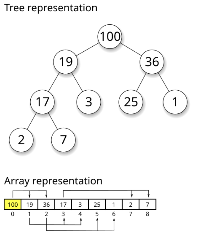
Heap Property

# Min-heap: Parent ≤ Children
#       1
#      / \
#     3   2
#    / \ / \
#   8  5 7  9

# Root always has minimum value
# Height = log₂(n)

Key Benefits: * Fast access to min/max: O(1) * Fast insertion: O(log n) * Fast removal: O(log n)

Python Heap Example

import heapq  # Python's built-in heap implementation

# Create an empty min-heap
# Min-heap property: parent <= children
heap = []

# Add items - each push is O(log n)
# Heap automatically reorganizes to maintain property
heapq.heappush(heap, 5)
heapq.heappush(heap, 2)
heapq.heappush(heap, 8)
heapq.heappush(heap, 1)

print(heap)  # [1, 2, 8, 5] - partially ordered

# Get and remove minimum - O(log n)
# Heap reorganizes after removal
min_val = heapq.heappop(heap)
print(min_val)  # 1 (smallest element always at top)

# Heap automatically maintains order after each operation!

When to Use Heaps

Important

Perfect Use Cases:

🏥 Priority Queues - Process items by importance
📊 Finding Top-K Elements - Get k largest/smallest efficiently
🎮 Event Scheduling - Handle events in time order
🚗 Route Planning - Dijkstra’s shortest path algorithm
📈 Streaming Data - Maintain running median/statistics

Trade-off: Not fully sorted, just maintains priority relationship

Part 4: O(2^n) - Exponential Time

The Recursive Monster 💥

O(2^n) means time doubles with each additional element!

Warning: Exponential algorithms become impossible very quickly. Even 50 items can take longer than the age of the universe!

What is O(2^n) - Exponential Time?

The Recursive Explosion 💥

O(2^n) means the algorithm’s time doubles with each additional input!

Real-World Analogy: * Like a chain letter - each person sends to 2 more * Day 1: 1 person, Day 2: 2, Day 3: 4… * Day 30: Over 1 billion people!

Explosive Growth 🚀

10 items → 1,024 operations
20 items → 1,048,576 operations
30 items → 1,073,741,824 operations
Each +1 item doubles the work!

Key Insight 🔑

Typically uses branching recursion - each call creates multiple recursive calls.

Danger Signal:

“Does my function call itself multiple times?”

If yes → Might be O(2^n)!

Naive Fibonacci - Classic O(2^n)

The Exponential Fibonacci

def fibonacci(n):
    """Naive recursive Fibonacci - O(2^n) exponential time!"""
    # Base case: fib(0) = 0, fib(1) = 1
    if n <= 1:
        return n
    
    # TWO recursive calls - this creates exponential growth!
    # Each call branches into two more calls
    return fibonacci(n-1) + fibonacci(n-2)

# The explosion:
# fib(5) calls fib(4) and fib(3)
# fib(4) calls fib(3) and fib(2)
# fib(3) is calculated MULTIPLE times! (wasteful redundancy)

print(fibonacci(10))  # Result: 55
# But took ~177 function calls to compute!
# Time complexity: O(2^n) - doubles with each n

Why O(2^n)? * Each call creates 2 more calls * Massive redundant computation * Binary tree of recursion

The O(n) Solution

def fibonacci_fast(n):
    """Iterative Fibonacci - O(n) linear time!"""
    # Base case
    if n <= 1:
        return n
    
    # Iterative approach: O(n)
    # Only stores two previous values
    prev, curr = 0, 1
    # Build up from fib(2) to fib(n)
    for _ in range(2, n + 1):
        prev, curr = curr, prev + curr  # Simultaneous assignment
    return curr

# OR use memoization (caching)
from functools import lru_cache

@lru_cache(maxsize=None)  # Cache all results
def fib_memo(n):
    """Memoized Fibonacci - O(n) with caching"""
    if n <= 1:
        return n
    # Same recursive structure, but results are cached
    return fib_memo(n-1) + fib_memo(n-2)

# Now each fib(k) computed only once!
print(fibonacci_fast(50))  # Instant! No exponential explosion

Interactive Fibonacci Demo

Watch the Exponential Explosion! 🎮

See how naive Fibonacci creates massive redundant calculations!

Naive Fibonacci - O(2^n) Recursive Explosion

Calculating: Ready to calculate!
Function Calls: 0 | Depth: 0 | Result: -
Status: Choose a Fibonacci number to calculate

Mini Challenge: Optimization Challenge

Compare O(2^n) vs O(n)! 🧑‍💻

Challenge: Fibonacci Performance

import time  # For timing execution
from functools import lru_cache  # For memoization decorator

# Naive O(2^n) - exponential time complexity
def fib_slow(n):
    """Naive recursive Fibonacci without caching"""
    if n <= 1:
        return n
    # Each call creates 2 more calls - exponential growth!
    return fib_slow(n-1) + fib_slow(n-2)

# Optimized O(n) with memoization (caching)
@lru_cache(maxsize=None)  # Decorator caches all results
def fib_fast(n):
    """Optimized Fibonacci with memoization"""
    if n <= 1:
        return n
    # Same structure, but cached results prevent recalculation
    return fib_fast(n-1) + fib_fast(n-2)

# Test both approaches with different input sizes
test_values = [10, 15, 20, 25, 30]

print("n\tSlow Time\tFast Time\tSpeedup")
for n in test_values:
    # Time slow version (O(2^n))
    start = time.time()
    result_slow = fib_slow(n)
    slow_time = time.time() - start
    
    # Time fast version (O(n))
    fib_fast.cache_clear()  # Clear cache for fair comparison
    start = time.time()
    result_fast = fib_fast(n)
    fast_time = time.time() - start
    
    # Calculate speedup factor
    speedup = slow_time / max(fast_time, 0.000001)  # Avoid division by zero
    print(f"{n}\t{slow_time:.4f}s\t\t{fast_time:.6f}s\t{speedup:.0f}x")
    
    # Stop if slow version takes too long
    if slow_time > 5:
        print("Stopping - exponential version too slow!")
        break

# YOUR TASK: What patterns do you notice?
# How does the speedup change as n increases?
# Notice: speedup grows exponentially!

Part 5: Travelling Salesman Problem

The Ultimate Optimization Challenge 🗺️

Finding the shortest route through all cities!

What is the Travelling Salesman Problem?

The Ultimate Route Challenge 🗺️

The Problem: Visit every city exactly once and return home using the shortest possible route.

Real-World Applications:

🚚 Delivery Services - UPS saves millions optimizing routes
🏭 Circuit Board Manufacturing - Drilling holes efficiently
🧬 DNA Sequencing - Optimal gene arrangements
🚌 School Bus Routes - Getting kids to school faster

Why It Matters 🚚

Amazon saves fuel and time
Manufacturing saves money
Everyone gets faster service
Reduces carbon emissions

The Challenge ⚡

3-4 cities: Easy
10 cities: 3,628,800 routes!
20 cities: More routes than atoms in universe!
Optimal solution: O(n!) factorial time

Key Question: How do we find good routes without checking every possibility?

TSP Complexity: The Factorial Explosion

Important

For n cities, there are (n-1)!/2 unique routes

Why? Fix starting city, divide by 2 (clockwise/counterclockwise are same).

The Numbers

import math  # For factorial calculation

def tsp_routes(n):
    """Calculate number of unique TSP routes for n cities"""
    if n <= 1:
        return 0
    # Formula: (n-1)! / 2
    # Fix start city, divide by 2 (clockwise = counterclockwise)
    return math.factorial(n-1) // 2

# Watch the factorial explosion!
for n in range(3, 11):
    routes = tsp_routes(n)
    print(f"{n} cities: {routes:,} routes")
    # Notice: each additional city multiplies routes dramatically!

Results:

3 cities → 1 route, 5 cities → 12 routes
10 cities → 181,440 routes, 15 cities → 43,589,145,600 routes!

Time to Check All Routes

Assuming 1 microsecond per route:

10 cities: 0.18 seconds ✓
15 cities: 12 hours ⚠️
20 cities: 77 years 🛑
25 cities: 490 billion years! 💀

Reality: Need smart approximations, not exhaustive search!

Interactive TSP Demo

Plan Your Route! 🎮

Click on the map to add cities, then find the best route!

🗺️ Interactive Travelling Salesman Demo

Cities: 0
Possible Routes: 0
Best Distance: -
Computation Time: -
⚠️ Complexity: Add cities!

Mini Challenge: TSP Approximations

Smart Route Planning! 🧑‍💻

Challenge: Nearest Neighbor Heuristic

import random  # For generating random city positions
import math    # For distance calculations

# Generate random cities in a 100x100 grid
def generate_cities(n):
    """Create n cities with random (x, y) coordinates"""
    return [(random.randint(0, 100), 
             random.randint(0, 100)) 
            for _ in range(n)]

# Calculate Euclidean distance between two cities
def distance(city1, city2):
    """Calculate straight-line distance between cities"""
    x1, y1 = city1
    x2, y2 = city2
    # Pythagorean theorem: sqrt((x2-x1)^2 + (y2-y1)^2)
    return math.sqrt((x2-x1)**2 + (y2-y1)**2)

# Nearest neighbor heuristic - O(n²) approximation algorithm
def nearest_neighbor(cities):
    """Greedy TSP approximation: always visit nearest unvisited city"""
    unvisited = cities.copy()  # Copy to avoid modifying original
    route = [unvisited.pop(0)]  # Start at first city
    
    # Continue until all cities visited
    while unvisited:
        current = route[-1]  # Current city is last in route
        # Find nearest unvisited city using min() with key function
        nearest = min(unvisited, 
                      key=lambda c: distance(current, c))
        route.append(nearest)  # Add to route
        unvisited.remove(nearest)  # Mark as visited
    
    # Return to start city to complete the tour
    route.append(route[0])
    return route

# Calculate total distance of a route
def route_distance(route):
    """Sum distances between consecutive cities in route"""
    total = 0
    # Add distance between each pair of consecutive cities
    for i in range(len(route) - 1):
        total += distance(route[i], route[i+1])
    return total

# Test it!
cities = generate_cities(10)  # Create 10 random cities
route = nearest_neighbor(cities)  # Find approximate route
dist = route_distance(route)  # Calculate total distance

print(f"Route distance: {dist:.2f}")
print("Route:", route)

# Not optimal, but fast O(n²) and reasonably good!
# Avoids O(n!) brute force - practical for real-world use

Complexity Comparison Summary

Choosing the Right Algorithm

Complexity	Name	Example	10 items	1000 items	When to Use
O(1)	Constant	Dict lookup	1 step	1 step	Direct access possible
O(log n)	Logarithmic	Binary search	3 steps	10 steps	Data is sorted
O(n)	Linear	Simple search	10 steps	1000 steps	Must check each item
O(n log n)	Log-linear	Merge sort	33 steps	10,000 steps	Good general sorting
O(n²)	Quadratic	Bubble sort	100 steps	1,000,000 steps	Small datasets only
O(2^n)	Exponential	Naive Fibonacci	1024 steps	Impossible	Avoid if possible!
O(n!)	Factorial	TSP (brute force)	3.6M steps	Impossible	Need approximations

Key Takeaways

Important

What We Learned Today:

⚡ O(1) - Hash tables give instant access regardless of data size
🔍 O(log n) - Binary search and heaps scale beautifully through divide-and-conquer
🏥 Heaps - Maintain priority order with O(log n) operations
💥 O(2^n) - Exponential algorithms become impossible quickly - use memoization!
🗺️ TSP - Real-world problems often require smart approximations, not perfect solutions
📊 Trade-offs - Choose algorithms based on data size, structure, and requirements

Tip

The Big Picture: Understanding complexity helps you write efficient code that scales. Small algorithmic choices make huge differences in real-world performance!

Next Steps & Practice

Note

To Continue Learning About Complexity 🤔:

📚 Study more sorting algorithms (merge sort, quick sort, heap sort)
🔬 Analyze algorithms in your own code
💻 Practice on coding platforms (LeetCode, HackerRank)
🎯 Learn about dynamic programming (turns O(2^n) → O(n))
🚀 Explore graph algorithms (Dijkstra, A*, etc.)

Remember: The best algorithm depends on your specific problem, data size, and constraints. There’s no one-size-fits-all solution!